
A master production schedule (MPS) states which end items a plant will build, in what quantities, in which weekly periods, over a horizon of several months. It sits between the aggregate S&OP production plan and the MRP run: the production plan speaks in families and months, the MPS translates that into buildable items and weeks, and MRP explodes those decisions into component orders. The schedule is a commitment, not a forecast; once inside the frozen fence, it is what the plant has promised to do.
This guide walks the mechanics with a full eight-week example: projected available balance, when an MPS quantity fires, and how available-to-promise is computed line by line. All of it can be recomputed by hand, which is also the test any MPS spreadsheet or ERP configuration should pass before anyone trusts it.
Where the MPS sits in the planning stack
The MPS occupies the middle altitude of the planning stack: below the aggregate S&OP production plan, above MRP and the shop-floor schedule. Four plans get confused with each other in most plants, and each answers a different question at a different granularity:
| Plan | Unit of planning | Time bucket | Horizon | Question it answers |
|---|---|---|---|---|
| Production plan (S&OP) | Product family | Month | 12–36 months | What volume will we run per family? |
| Master production schedule | End item or model | Week | 3–12 months | Which items, how many, which weeks? |
| Material requirements plan (MRP) | Component and material | Week or day | Driven by MPS | What to order and make, and when? |
| Detailed production schedule | Job, line, and shift | Day or hour | Days to weeks | Which order runs on which resource next? |
The discipline flows downhill. The MPS must sum to the approved family volumes from the S&OP process, stay inside the capacity envelope tested by rough cut capacity planning and the supply review, and feed MRP through accurate bills of material. Break any of those three connections and the schedule becomes a document about a plant that does not exist.
What the MPS consumes
Five inputs drive the calculation: the demand forecast per item per week, booked customer orders, on-hand inventory, lot-sizing rules, and the planning time fences. Forecast quality upstream matters exactly as much here as it did in the demand meeting; a schedule built on a biased forecast inherits the bias as inventory or shortages, which is why the manufacturing sales forecasting process and the MPS are the same conversation four weeks apart.
In each weekly bucket, the demand the schedule nets against is the greater of forecast and booked orders (the common convention; some systems switch to orders-only inside a demand time fence). Wikipedia’s MPS entry lists the same core inputs and adds the practical warning that the MPS plans what production can and will do, not raw demand.
A worked 8-week MPS example
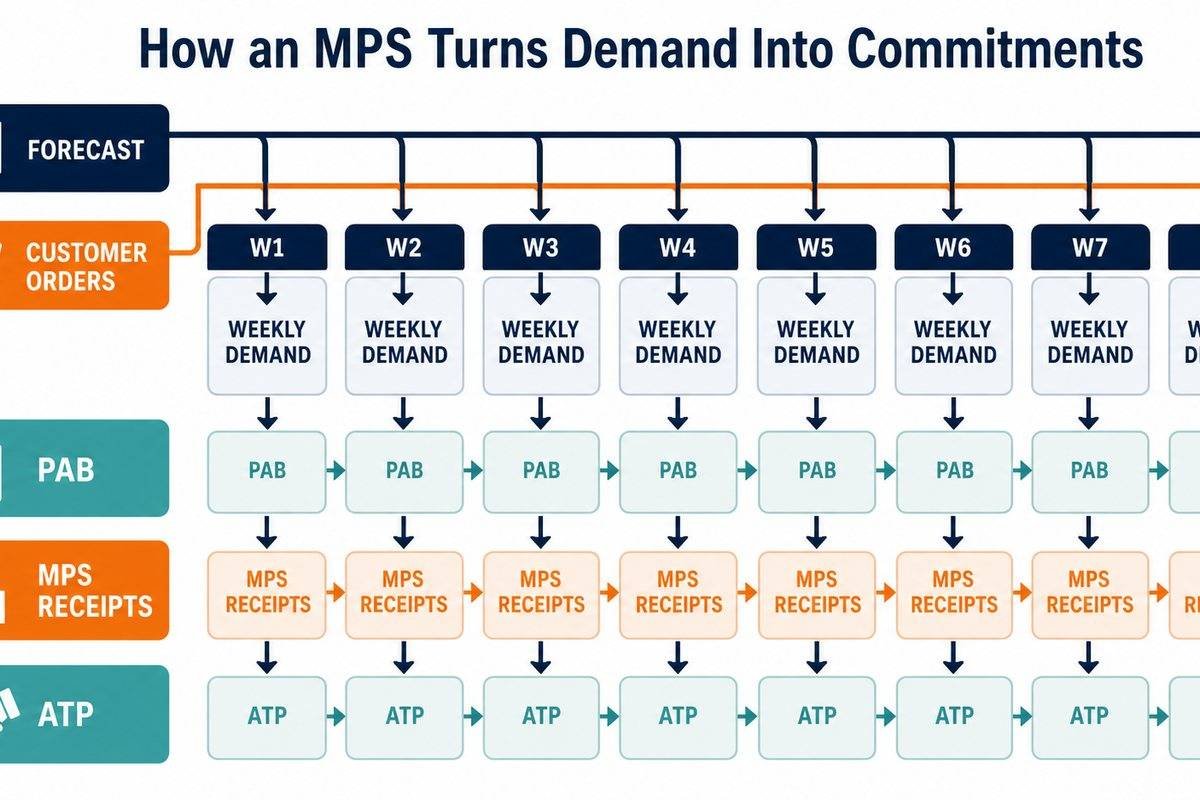
The table below is an illustrative example for one pump model, PF-100. Opening inventory is 1,200 units, the lot size is a fixed 1,500, safety stock is zero, and forecast steps up from 600 to 800 units per week in week 5. Booked orders taper off as the horizon extends, which is the normal shape: near weeks are mostly orders, far weeks mostly forecast.
| W1 | W2 | W3 | W4 | W5 | W6 | W7 | W8 | |
|---|---|---|---|---|---|---|---|---|
| Forecast | 600 | 600 | 600 | 600 | 800 | 800 | 800 | 800 |
| Customer orders | 750 | 500 | 300 | 150 | 100 | 0 | 0 | 0 |
| Projected available balance | 450 | 1,350 | 750 | 150 | 850 | 50 | 750 | 1,450 |
| MPS receipt | — | 1,500 | — | — | 1,500 | — | 1,500 | 1,500 |
| Available-to-promise | 450 | 550 | — | — | 1,400 | — | 1,500 | 1,500 |
Tracing the projected available balance (PAB) row, where weekly demand is the greater of forecast and orders:
- W1: demand is max(600, 750) = 750. PAB = 1,200 − 750 = 450. Positive, so no MPS fires.
- W2: demand 600. 450 − 600 would go negative, so an MPS lot of 1,500 fires. PAB = 450 + 1,500 − 600 = 1,350.
- W3: 1,350 − 600 = 750. W4: 750 − 600 = 150.
- W5: demand steps to 800. 150 − 800 goes negative, so another lot fires: 150 + 1,500 − 800 = 850.
- W6: 850 − 800 = 50. W7: lot fires: 50 + 1,500 − 800 = 750. W8: lot fires: 750 + 1,500 − 800 = 1,450.
Week 8 ends at 1,450 units, nearly a full lot of inventory, purely because a fixed 1,500 lot meets an 800-per-week demand. That leftover is not a calculation error; it is the lot-sizing policy made visible, and it is the kind of number that should flow back into the next lot-size discussion.
Available-to-promise (ATP) uses the discrete method: each ATP covers the window from one MPS receipt to just before the next, counting only booked orders, because forecast is not a promise to a specific customer.
- W1 ATP = on hand 1,200 − orders before the first receipt (W1’s 750) = 450.
- W2 ATP = 1,500 − orders in W2–W4 (500 + 300 + 150) = 550.
- W5 ATP = 1,500 − orders in W5–W6 (100 + 0) = 1,400.
- W7 and W8 ATP = 1,500 each, with no booked orders yet against those lots.
When a customer calls asking for 600 units in week 3, the answer comes off this row: W1’s 450 plus W2’s 550 covers it without touching the schedule. Sales commitments made against ATP leave the MPS stable; commitments made against hope get expedited later.
Time fences: frozen, slushy, liquid

The horizon splits into three zones by how much change is allowed. Inside the frozen fence (commonly the cumulative lead time of the product, often two to four weeks), the schedule changes only by exception with management sign-off, because material is committed and capacity is loaded. The slushy zone allows mix changes within the approved volume: swapping one model for another that consumes similar capacity and components. The liquid zone beyond that is planning space, where the schedule can move freely.
The fences are a management contract, not a system setting. A plant where sales routinely breaks the frozen fence has no MPS; it has a suggestion box with weekly buckets. The honest fix is rarely freezing harder: it is shortening lead times until the frozen zone the business needs matches the one it can tolerate.
Building the schedule, then keeping it honest
Standing up an MPS from scratch follows a repeatable sequence, described in similar terms by ProjectManager’s MPS guide: select the items to master-schedule, disaggregate the S&OP family plan into those items, load current inventory and booked orders, apply lot sizes and fences, and compute PAB, receipts, and ATP as above. Two practices keep the result trustworthy past the first month:
- Weekly maintenance at fixed altitude. The master scheduler replans the liquid zone, adjusts the slushy zone within S&OP volume, and documents every frozen-zone exception with its cost. The list of exceptions is a better management report than the schedule itself.
- Measure schedule stability. Track the percentage of MPS quantities inside the frozen fence that changed after commitment. Rising instability is an early symptom: of a biased forecast, an optimistic supply review, or a fence the organization does not respect.
Component data quality decides whether MRP amplifies the schedule or its errors: the explosion is only as good as the accuracy of the bills of material underneath it.
Master production schedule FAQ
What is a master production schedule in simple words?
A master production schedule is the plant’s build list: which products, how many, in which weeks. It converts the monthly volume agreed in S&OP into weekly commitments the factory schedules against, and it drives the material system that orders every component underneath.
How do you calculate a master production schedule?
Week by week, subtract demand (the greater of forecast and booked orders) from the projected available balance; when the balance would fall below zero or safety stock, schedule a receipt of the lot size and add it in. The eight-week PF-100 table above runs this arithmetic in full.
What is the difference between a master schedule and a production schedule?
The master production schedule plans end items in weekly buckets over months and is the contract between sales, planning, and the plant. The detailed production schedule sequences specific jobs on specific machines and shifts over the next days, executing what the MPS committed.
What is MPS in SAP and other ERP systems?
In SAP and comparable ERP systems, MPS is a planning run restricted to designated master-scheduled items, executed before full MRP so critical end items are planned under tighter control first. The logic mirrors the manual arithmetic above; the configuration decisions that matter are lot size, fences, and which items make the MPS list.
Next steps
- Rebuild one item’s MPS by hand for eight weeks, the way the PF-100 table does, and compare against what your system generated; any difference is a lot size, fence, or demand-netting setting you did not know you had.
- Publish the ATP row to whoever answers customer date requests, and route promises through it for one month.
- Start tracking frozen-zone changes this cycle; the count, and who caused each, is the fastest diagnosis of whether the schedule is a commitment or a suggestion.