
Dave Garwood’s archived RDGarwood articles treated sales forecasting as a management process, not a statistical contest. The recurring idea was practical: create one accountable view of demand, test it against manufacturing reality, and reduce the parts of the business that depend on a forecast when demand cannot be predicted reliably.
This article reconstructs and expands that approach from historical RDGarwood pages. It is an editorial analysis for today’s planners, not a statement from a currently operating Garwood consultancy and not an attempt to recreate the former team.
The core idea: forecast decisions, not just demand
Sales forecasting in manufacturing estimates what customers are likely to buy over a defined horizon. The forecast should then drive decisions about raw materials, labor, equipment, suppliers, inventory, cash, and promised delivery dates. A number that never changes one of those decisions is reporting, not planning.
That distinction explains why a revenue forecast from a CRM is rarely enough for a factory. Manufacturing needs units, product families, configuration, timing, location, and uncertainty. A $1 million opportunity could represent one capacity-intensive custom machine or thousands of standard parts; the production implications are completely different.
IBM’s overview of sales forecasting similarly connects forecasts with production, inventory, staffing, and budgeting. The Garwood archive pushed the operational question further: what action should the company take when the number is uncertain?
What can be recovered from the historical Garwood method?
Several archived RDGarwood articles, preserved in the Wayback Machine’s copy of the original article index, form a coherent method even though they were originally published separately. “Making a Better Sales Forecast” argued for demand planning with one set of numbers, defined demand streams, named accountability, and regular actual-versus-plan review. “A Remedy for Your Forecast Headache!” challenged teams to reduce their exposure to forecasting through lead-time reduction, common components, postponement, and make-to-order policies. Other articles connected the demand view to supply review and executive S&OP decisions.
Combined, those ideas create five operating principles:
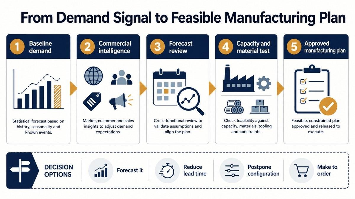
- Start with a statistical baseline, then show judgment separately. A planner should be able to see what the model produced and which commercial assumptions changed it.
- Give each demand stream an owner. Base demand, promotions, major accounts, new products, and one-time projects behave differently and should not disappear inside one total.
- Review error for learning, not blame. Compare actual demand with the forecast, find the assumption that failed, and update the process.
- Translate the forecast into a feasible plan. Capacity, materials, tooling, labor, and supplier constraints must be tested before the business commits.
- Remove avoidable forecast dependence. Some uncertainty is better handled by a shorter lead time or a different product and fulfillment design than by a more elaborate model.
Should every manufactured item be forecast?
No. The first decision is whether an item should be forecast at all. Stable, repeated demand can support a time-series forecast. Irregular, high-value, highly configurable, or project-driven demand may be better managed through make-to-order rules, customer commitments, capacity reservations, or common-component planning.
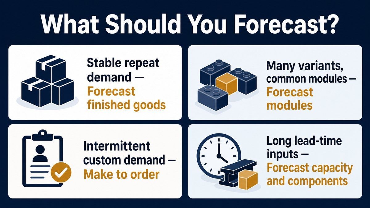
| Demand and product condition | Preferred planning response | Why |
|---|---|---|
| Stable repeat demand, short replenishment cycle | Forecast finished goods or product families | History provides a usable baseline and inventory can absorb normal error. |
| Intermittent demand for expensive configurations | Make to order; forecast shared capacity and long-lead components | Finished-goods error is costly, while common inputs still need advance planning. |
| Many variants built from common modules | Forecast modules; postpone final configuration | Pooling demand at the common level reduces SKU-level uncertainty. |
| Customer has a credible schedule or blanket order | Use customer commitments with a consumption rule | The direct signal may be more informative than extrapolating shipment history. |
| Lead time exceeds customers’ tolerance | Forecast only the portion that cannot be replenished in time | Reducing cumulative lead time shrinks the horizon exposed to forecast error. |
This is one of the strongest information gains in the archived approach. A forecast is not automatically the right control mechanism. Before investing in another model, ask whether the product architecture, fulfillment policy, or lead time is forcing the company to predict farther ahead than necessary.
How do you build a manufacturing sales forecast?
A practical process has seven steps. The sequence keeps facts, judgment, and constraints visible instead of blending them into an unexplained spreadsheet total.
1. Define the decision and planning level
Choose the unit of measure, hierarchy, location, time bucket, and horizon. Product-family volume may be right for monthly sales and operations planning; individual SKUs and weekly buckets may be necessary for replenishment. Do not measure accuracy at a more aggregated level than the decision it supports.
2. Build clean demand history
Separate true customer demand from shipments distorted by stockouts, allocation, returns, internal transfers, or order batching. A shipment of zero during a stockout does not prove that demand was zero. Mark promotions, price changes, lost customers, and exceptional projects so the baseline does not learn from events that will not repeat.
3. Create a baseline by segment
Use a method that fits the demand pattern. Moving averages or exponential smoothing can suit stable items; seasonal models suit repeated seasonal demand; causal models can incorporate price or market drivers; new products need analogs, customer research, or scenario ranges. There is no universally best forecasting method for manufacturing.
4. Add commercial intelligence as named assumptions
Sales and marketing should contribute known account changes, pipeline, promotions, competitive events, and launches. Record each override with an owner, reason, start and end date, and expected unit effect. That audit trail lets the team learn whether overrides improve the baseline.
5. Reconcile one demand plan
Resolve duplicate account input and distinguish an unconstrained demand forecast from a sales target. A target describes an ambition; a forecast describes the most likely demand under stated assumptions. Treating the target as the forecast quietly transfers an aspiration into inventory and capacity commitments. The consensus meeting where these conflicts get resolved is detailed in the demand review process guide.
6. Test capacity and material feasibility
Translate the demand plan through bills of material, routings, yields, batch sizes, supplier lead times, and plant constraints. Produce options for gaps: inventory build, overtime, subcontracting, allocation, alternate materials, promotion timing, or a revised service promise. The master data this translation depends on is what the ERP readiness checklist audits.
7. Measure, explain, and learn
Review forecast error and forecast bias at the same level and lag used when the original decision was made. Compare baseline accuracy with final forecast accuracy. If manual overrides repeatedly make the result worse, change the override rule rather than asking for more confident commentary. Metric choices for this review, from WAPE to tracking signals, are compared in the forecast accuracy metrics guide.
Manufacturing sales forecast example
Consider a manufacturer planning a pump family. Its baseline for October is 1,000 units. Sales identifies a confirmed customer ramp of 180 units and a promotion expected to add 120, while a distributor reports a likely 80-unit reduction. The unconstrained demand forecast becomes 1,220 units.
| Forecast component | Units | Assumption owner |
|---|---|---|
| Statistical baseline | 1,000 | Demand planning |
| Confirmed account ramp | +180 | Key-account sales |
| Promotion uplift | +120 | Marketing |
| Distributor reduction | −80 | Channel sales |
| Unconstrained demand | 1,220 | Demand review |
The plant can make 1,100 units in October, and all components except one common seal are available for that volume. On-hand seals plus confirmed receipts cover 1,000 assemblies; the remaining seals have a ten-week replenishment lead time. The team therefore approves 1,100 finished pumps, reserves 120 units of customer demand for November delivery, and expedites exactly 100 seals to close the October material gap for the highest-margin segment. The forecast did not become more accurate during the meeting; the business became more prepared.
How does the forecast connect to S&OP and production planning?
The demand forecast should enter S&OP as an unconstrained view of demand. Supply review converts it into feasible scenarios. Finance evaluates revenue, margin, inventory, and cash consequences. Executives then approve one plan and its exceptions. Oracle’s S&OP explanation describes the process as aligning demand, supply, and financial planning across strategic and tactical horizons.
After approval, aggregate S&OP volumes guide the master production schedule, material requirements planning, purchasing, staffing, and supplier schedules. The forecast and the production plan should not be confused: the first expresses expected demand; the second states what the company has decided it can and will supply.
Five ways to reduce forecast exposure
The old “forecast headache” article — still readable through the archived index linked above — remains useful because it treats uncertainty as a design problem. Manufacturers can often reduce risk through five levers:
- Classify unforecastable items. Move genuinely intermittent or custom products toward make-to-order controls.
- Reduce end-to-end lead time. Faster replenishment means fewer weeks of demand must be predicted before action can be taken.
- Increase component commonality. Forecast pooled demand for shared modules instead of guessing every finished configuration.
- Postpone differentiation. Hold semi-finished inventory and configure color, packaging, firmware, or accessories after demand is clearer.
- Use customer plans carefully. Blanket orders and customer schedules can improve visibility when ownership, update frequency, and consumption rules are explicit.
These changes do not eliminate planning. They move planning to a level where uncertainty is lower and response is faster.
Common failures and the corrective rule
| Failure | What it causes | Corrective rule |
|---|---|---|
| Forecast equals the sales target | Systematic optimism and excess commitments | Keep target, baseline, and final forecast as separate fields. |
| One total hides demand streams | No one can explain the variance | Assign owners to base, promotion, account, project, and launch demand. |
| Accuracy is reviewed without bias | Consistent over- or under-forecasting can cancel inside averages | Track both magnitude and direction of error. |
| Forecast changes after actuals arrive | Reported accuracy becomes meaningless | Freeze the forecast version at each decision lag. |
| Every SKU receives the same method | High effort and poor fit | Segment by value, variability, lifecycle, and fulfillment policy. |
Manufacturing sales forecasting FAQ
How accurate should a manufacturing sales forecast be?
There is no universal target, and chasing one usually backfires. Accuracy depends heavily on the level being measured: a product-family forecast one month out can be very reliable while the SKU-week forecasts underneath it are individually poor. Benchmark against your own frozen baseline at the decision level and lag, and judge improvement against that history rather than an industry number.
When should an item be make-to-stock instead of make-to-order?
Make-to-stock fits items with stable, repeated demand and replenishment cycles shorter than the delivery promise. Make-to-order fits expensive, highly configured, or genuinely intermittent items where holding finished stock is costly and customers accept the lead time. The decision table earlier in this article maps the in-between cases: forecast common modules, postpone final configuration, or plan against customer schedules.
What is the difference between a sales target and a sales forecast?
A target is an ambition used to motivate and measure the commercial team. A forecast is the most likely demand under stated assumptions. The two numbers can legitimately differ — and the moment a target is silently entered as the forecast, the gap turns into unplanned inventory or missed deliveries.
The practical takeaway
The most durable part of Dave Garwood’s archived approach is the refusal to treat forecast accuracy as the end goal. A manufacturing forecast earns trust when assumptions are visible, demand streams have owners, bias is confronted, constraints are tested, and the resulting plan changes real actions.
Start with one product family and one frozen monthly forecast. Separate the baseline from overrides, trace the result into capacity and material decisions, and identify one place where shorter lead time or delayed configuration can reduce forecast dependence. That small operating loop will reveal more than another debate about which forecasting formula is supposedly best.