
The tracking signal formula is the running sum of forecast errors divided by the mean absolute deviation: TS = RSFE ÷ MAD. The result says how far a forecast has drifted in one direction, measured in units of its own typical error. A value near zero means errors are balancing out; a value beyond about ±4 means the forecast is leaning hard enough that the drift is unlikely to be noise.
The formula takes one line. The disagreements start at the control limit, where different references defend ±3, ±3.75, and ±4 without explaining why they differ. They are not contradicting each other; they are choosing different points on the same statistical trade-off, and seeing that derivation once removes the confusion permanently.
What the tracking signal measures
A tracking signal monitors forecast bias relative to forecast noise. Cumulative error alone cannot do this job: a +500-unit drift is alarming on a product that misses by 50 units in a typical month and irrelevant on one that misses by 5,000. Dividing by MAD rescales the drift so one control limit works across items of any size.
That makes the tracking signal a monitoring tool, not a diagnosis. It rings the bell; finding out whether a stale promotion override, a lost customer, or a slow model caused the drift is the work described in the guide to forecast bias, which this metric exists to detect early.
The tracking signal formula, step by step
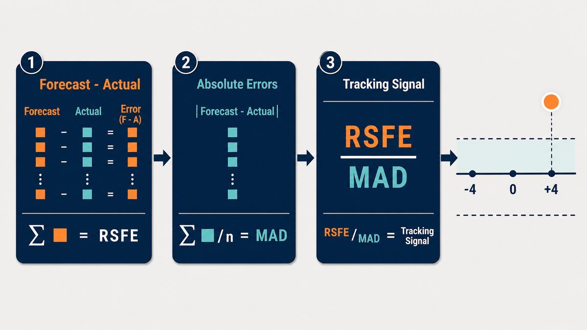
Three quantities build the signal, computed fresh each period:
Forecast error = Forecast − Actual (this site’s convention throughout: positive means over-forecasting; some references use Actual − Forecast, which flips every sign, so label whichever you adopt).
RSFE = running sum of forecast errors, signed, so offsetting errors cancel.
MAD = mean absolute deviation: the average of the absolute errors to date.
Tracking signal = RSFE ÷ MAD, recomputed every period as both numerator and denominator update. The units cancel, leaving a pure number that reads as “how many typical errors of drift have accumulated.”
A worked example: eight months, one drifting forecast
The dataset below is an illustrative example built to be recomputed by hand. A planner freezes a forecast of 1,000 units every month while real demand slowly erodes:
| Month | Forecast | Actual | Error (F − A) | RSFE | |Error| | MAD to date | Tracking signal |
|---|---|---|---|---|---|---|---|
| 1 | 1,000 | 980 | +20 | +20 | 20 | 20.0 | +1.0 |
| 2 | 1,000 | 1,020 | −20 | 0 | 20 | 20.0 | 0.0 |
| 3 | 1,000 | 950 | +50 | +50 | 50 | 30.0 | +1.7 |
| 4 | 1,000 | 940 | +60 | +110 | 60 | 37.5 | +2.9 |
| 5 | 1,000 | 930 | +70 | +180 | 70 | 44.0 | +4.1 |
| 6 | 1,000 | 960 | +40 | +220 | 40 | 43.3 | +5.1 |
| 7 | 1,000 | 920 | +80 | +300 | 80 | 48.6 | +6.2 |
| 8 | 1,000 | 910 | +90 | +390 | 90 | 53.8 | +7.3 |
Spot-checking month 5: RSFE = 20 − 20 + 50 + 60 + 70 = +180; cumulative absolute error = 20 + 20 + 50 + 60 + 70 = 220, so MAD = 220 ÷ 5 = 44; tracking signal = 180 ÷ 44 = +4.1. Every other row recomputes the same way.
The story the column tells is the point of the tool. Months 1 and 2 look like healthy noise. The signal wakes at +2.9 in month 4, crosses the common ±4 limit in month 5, and by month 8 sits at +7.3, with the forecast now missing high eight months into a demand decline it never acknowledged. A monthly error report would have shown each miss individually; only the running ratio shows them compounding in one direction.
What is an acceptable tracking signal range?
Common control limits are ±3, ±3.75, and ±4, and the spread has a statistical origin, not an editorial one. For approximately normal forecast errors, one standard deviation equals roughly 1.25 MAD. The limits translate as:
| Limit in MAD | Approx. in standard deviations | Character |
|---|---|---|
| ±3 | ≈ 2.4σ | Sensitive: catches drift early, more false alarms |
| ±3.75 | ≈ 3.0σ | The classic three-sigma control chart translated into MAD |
| ±4 | ≈ 3.2σ | Conservative: fewer alarms, later detection |
Practitioner references such as Value Chain Planning’s tracking signal example pick 3.75 MAD for exactly this reason: it is the three-sigma limit expressed in MAD units. Tighter limits suit expensive drift (capacity commitments, perishables); looser limits suit noisy, low-value items where chasing alarms costs more than the drift does. Pick per segment, write the limit on the report, and treat a breach as a trigger for investigation, never as an automatic model change.
Building it in Excel
With forecasts in B2:B13 and actuals in C2:C13, using row 5 as the example period:
- Error in D2: =B2-C2, filled down.
- RSFE in E5: =SUM(D$2:D5).
- MAD in F5: =AVERAGE(ABS(D$2:D5)) entered as an array formula, or the always-safe =SUMPRODUCT(ABS(D$2:D5))/ROWS(D$2:D5).
- Tracking signal in G5: =IFERROR(E5/F5,0), which returns 0 instead of an error before any demand history exists.
Conditional formatting on the signal column at your chosen limit turns the sheet into a working exception report for a handful of items; past a few hundred SKU-level signals, the calculation belongs in the planning system that already stores frozen forecasts.
Limits, variants, and when to reset
Three boundaries keep the tool honest. First, reset the signal after any deliberate model or process change: RSFE accumulated under the old model tells you nothing about the new one, and a stale running sum will ring alarms for months about a problem already fixed. Second, intermittent demand breaks the assumptions; MAD computed across mostly-zero periods is unstable, and the drift the signal detects may just be the item’s lumpiness. Use windowed measures from the forecast accuracy metrics guide instead. Third, a smoothed variant (exponentially weighted error divided by smoothed MAD, sometimes called Trigg’s method, noted in Wikipedia’s entry and its references) reacts faster to recent drift at the cost of a less intuitive number; the plain RSFE version is the right default for a monthly planning cycle.
Ownership matters more than the variant. A tracking signal breach should land on a named agenda, and the natural home is the scorecard segment of the monthly demand review, where the override owners who probably caused the drift are already in the room.
Tracking signal FAQ
How do you calculate a tracking signal?
Sum the signed forecast errors to date (RSFE), divide by the mean absolute deviation of those errors (MAD), and recompute both every period. With errors of +20, −20, +50, +60, and +70, RSFE is +180, MAD is 44, and the tracking signal is +4.1.
What is a tracking signal in forecasting?
A tracking signal is a control metric that detects persistent one-directional forecast error by comparing cumulative drift with typical error size. It answers whether a forecast is merely inaccurate, which is normal, or systematically leaning one way, which is fixable.
What is an acceptable range for a tracking signal?
Most references set control limits between ±3 and ±4 MAD. The values map to roughly 2.4 to 3.2 standard deviations for normal errors, so the choice trades early detection against false alarms; ±3.75 reproduces the classic three-sigma control limit.
What does a negative tracking signal mean?
Under the Forecast − Actual convention used here, a negative signal means persistent under-forecasting: actual demand keeps exceeding the forecast. Under the reverse convention it means the opposite, which is why the error formula belongs on every report that shows the number.
Next steps
- Add the four Excel columns to one product family’s frozen forecast history and read the signal’s trend, not just its latest value.
- Set limits per segment: tighter where drift is expensive, looser where demand is noisy, and write the chosen limit and error convention on the report.
- Route every breach to the demand review scorecard with a named owner, and reset the signal whenever the forecasting model genuinely changes.