
Rough cut capacity planning (RCCP) checks whether the master production schedule can be built by converting planned volumes into hours of load on a few critical resources and comparing that load with the hours those resources can actually deliver. It runs at product-family level over a monthly horizon, and it exists to catch a capacity hole three months out, when overtime and offloading are still options, instead of three weeks out, when only expediting is.
The technique is old, simple, and routinely skipped, usually because a plant assumes its ERP’s detailed capacity run covers the same ground. It does not: detailed capacity requirements planning (CRP) works after MRP has exploded every order and only for the near horizon. RCCP is the coarse, early check that decides whether that detailed run is worth performing on the schedule at all.
What rough cut capacity planning does
RCCP validates the master production schedule against critical resources before the schedule is released to MRP. It answers one question per resource per period: is the load the MPS implies within what this resource can demonstrably produce? Oracle’s long-standing manufacturing documentation describes RCCP as the check of the MPS against key resources, and that framing has not changed across ERP generations.
Two design choices define the method. First, it looks only at critical resources: the bottleneck cell, the paint line, the one qualified crew, a supplier’s committed weekly quantity. Modeling every work center at this stage recreates CRP with worse data. Second, it ignores lead-time offsets and work-in-process by default, treating a month’s schedule as a month’s load. That coarseness is deliberate; it makes the check fast enough to rerun for every scenario the supply review wants to test.
The RCCP formula
For each critical resource and each period:
Required hours = Σ (MPS quantity per family × standard hours per unit on that resource)
Available hours = demonstrated output hours the resource actually delivered on comparable months
Load % = Required ÷ Available × 100, with the gap in hours being Required − Available.
The word demonstrated carries the method. Nameplate capacity is what the equipment could theoretically do; demonstrated capacity is what the cell produced in the last six normal months, net of the changeovers, absenteeism, and maintenance that always happen. Plans built on nameplate look feasible and fail on the floor.
Three RCCP techniques and when each fits
Standard operations texts, echoed in Smartsheet’s overview, describe three ways to build the standard-hours factors that drive the formula:
| Technique | How the load factor is built | Accuracy | Fits when |
|---|---|---|---|
| Capacity planning using overall factors (CPOF) | Total historical hours per unit, spread across resources by historical percentage | Lowest | Stable mix, few resources, no routing data yet |
| Capacity bill (bill of resources) | Standard hours per unit per resource, taken from routings | Medium | Routings exist and mix varies by family; the usual default |
| Resource profile | Capacity bill plus lead-time offset, so hours land in the period they are consumed | Highest | Long cumulative lead times where load and schedule month differ |
Most manufacturers land on the capacity bill: accurate enough for family-level decisions, buildable from data the routing already holds. Move to resource profiles only when lead times are long enough that October’s schedule loads a component cell in September, because at that point the coarse version starts sending alarms to the wrong month.
A worked example: one cell, two families, four months
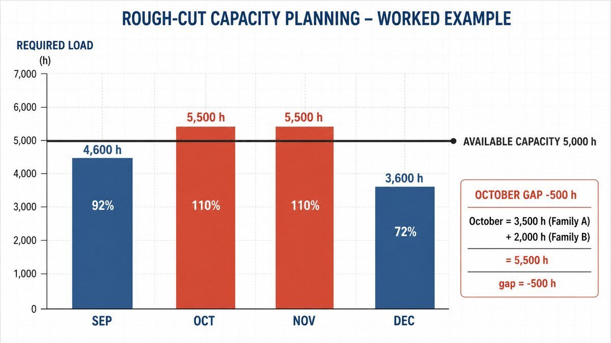
The figures below are an illustrative example built to be recomputed. A machining cell is the critical resource for two pump families. Standard hours per unit from the routings: family A 0.50 h, family B 0.80 h. Demonstrated capacity: 5,000 hours per month.
| Sep | Oct | Nov | Dec | |
|---|---|---|---|---|
| MPS family A (units) | 6,000 | 7,000 | 7,000 | 4,000 |
| MPS family B (units) | 2,000 | 2,500 | 2,500 | 2,000 |
| Load A (units × 0.50 h) | 3,000 | 3,500 | 3,500 | 2,000 |
| Load B (units × 0.80 h) | 1,600 | 2,000 | 2,000 | 1,600 |
| Required hours | 4,600 | 5,500 | 5,500 | 3,600 |
| Available hours | 5,000 | 5,000 | 5,000 | 5,000 |
| Load % | 92% | 110% | 110% | 72% |
| Gap (hours) | +400 | −500 | −500 | +1,400 |
Checking October: 7,000 × 0.50 = 3,500 hours for A, 2,500 × 0.80 = 2,000 hours for B, total 5,500 against 5,000 available, so the cell is loaded to 110% and short 500 hours. Across the four months the arithmetic nets to +800 spare hours, and the schedule is still infeasible in two of them; RCCP’s first lesson is always that quarterly averages hide monthly holes.
The 500-hour October gap converts back into units the way the planners think: 500 h ÷ 0.50 h = 1,000 units of family A, or 500 h ÷ 0.80 h = 625 units of family B. That conversion is what makes the result actionable. The options are the standard set: pull 400 hours of October work into September’s slack (leaving a 100-hour hole), add overtime, offload to a subcontractor, or reshape demand, and each option carries a price the supply review can attach.
RCCP vs capacity requirements planning
| RCCP | CRP | |
|---|---|---|
| Input | Master production schedule | MRP planned and released orders |
| Level | Product family, critical resources only | Every item, every work center |
| Horizon and bucket | Months, out to the planning horizon | Days or weeks, near term |
| Lead-time offset | Ignored (unless resource profiles) | Fully modeled |
| Question answered | Is this schedule roughly buildable? | Which orders overload which center, and when? |
RELEX’s planning guide draws the same line: CRP works the near weeks in weekly buckets, RCCP reaches out to the planning horizon in monthly ones. The two are sequential, not alternatives. RCCP clears the master production schedule for release; MRP explodes it; CRP then finds the detailed collisions the coarse check could never see.
Where the rough cut goes wrong
Three failures account for most bad RCCP results. Nameplate capacity in the available-hours line, which flatters every month. Standard hours from routings nobody has updated since the product launched, which is a bill of materials and routing accuracy problem before it is a capacity problem; the audit approach in the BOM accuracy guide extends to routings directly. And modeling too many resources, which turns a fifteen-minute check into a maintenance burden that quietly stops being run.
The boundary on the other side is real too. Plants with one product family and no genuine bottleneck get little from RCCP; a glance at total hours does the job. The method earns its place when mix shifts move load between resources and someone has to decide months ahead which promises the plant can keep.
Rough cut capacity planning FAQ
What is a rough cut capacity plan?
A rough cut capacity plan is the period-by-period comparison of hours required by the master production schedule against hours available on each critical resource, at product-family level. It flags months where load exceeds demonstrated capacity so the schedule can be adjusted before release.
What are the three types of capacity planning?
Manufacturing planning textbooks describe three levels: resource planning at the S&OP level over years, rough cut capacity planning at the MPS level over months, and capacity requirements planning at the MRP level over weeks. Each validates the plan produced one level above it.
What is RCCP in supply chain management?
RCCP is the feasibility gate between the demand-supply balance agreed in S&OP and the detailed material plan. It confirms that the volumes committed to customers can be produced by the resources most likely to constrain them, before purchasing and scheduling commit money to the plan.
What is the rough cut capacity planning formula?
Required hours equal MPS quantity multiplied by standard hours per unit, summed across families for each resource and period; load percent equals required hours divided by demonstrated available hours. A result above 100% is a capacity gap measured in hours, convertible back to units by dividing by the standard hours per unit.
Next steps
- Name the two to four resources that genuinely constrain the plant, and compute demonstrated hours for each from the last six normal months.
- Pull standard hours per unit per family from routings, and verify them against a recent build before trusting them.
- Build the load table for the current MPS horizon, mark every month above 100%, and take the hour gaps into the next supply review already converted to units and options.