
The components of aggregate production planning are production rate, workforce level, inventory and backlog, and the output unit you plan in, all set over a medium-term horizon of roughly 3 to 18 months. The choice of strategy comes down to which of these absorbs a swing in demand. Level planning holds production steady and lets inventory and backlog flex; chase planning moves workforce and output with demand; hybrid planning blends the two.
This fits a manufacturer or operations manager deciding how to respond to a seasonal or volatile demand signal before any order reaches the shop floor. The example below runs the same demand through all three strategies so you can see the tradeoff numerically, not just as a label.
What an aggregate production plan is
An aggregate production plan sets medium-term production volume, workforce, and inventory levels to match forecast demand before you commit to a detailed schedule. It answers how much to make, how many people you need, and how much stock to carry, at the level of product families rather than individual items.
You plan in aggregate units so you can reason about the whole facility instead of one product line. Because it runs ahead of execution, it is the layer that keeps a plant from re-planning its production planning vs production scheduling loop every time demand shifts by a few units. Aggregate planning sits above master scheduling and the shop floor, and it decides the broad levers that those lower levels then sequence.
The four components and what each one absorbs
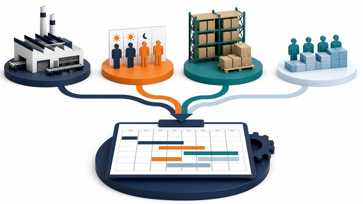
Every aggregate plan is built from four components, and each one exists to absorb a different part of the demand swing.
- Production rate: how many units you make per period. Holding this fixed is the level strategy; moving it is chase.
- Workforce level: the number of workers and how you flex it, through overtime, hiring, firing, or subcontracting.
- Inventory and backlog: how much finished stock you carry and how far you let orders wait when demand outpaces output.
- Output unit: the single measure you plan in, such as units, tons, or labor-hours, that lets you aggregate many products into one number.
Four things are needed to actually run aggregate planning: a logical overall unit for measuring output, a demand forecast for the planning interval, a statement of capacity, and a policy on workforce and subcontracting. Those four inputs map directly onto the four components above. ASCM, the operations-management body behind the APICS body of knowledge, treats this medium-term balancing as the bridge between sales and operations and the detailed schedule. A concise framing of the same taxonomy is on the Wikipedia page for aggregate planning.
Level, chase, and hybrid: what each strategy does
Level planning keeps output and workforce constant and lets inventory and backlog absorb the demand swing. Chase planning matches output to demand and keeps inventory lean by flexing the workforce. Hybrid planning holds a steady core and flexes only at the margin.
Level is cheapest to run when the cost of changing the workforce is high and holding stock is cheap. The downside is that inventory builds during low demand and backlogs or stockouts appear during peaks. Chase avoids holding stock but pays for hiring, firing, overtime, and the morale cost of an unstable headcount. Hybrid tries to keep the level most of the time and use overtime or limited chase only when demand moves outside a preset band.
The three strategies also behave differently on the shop floor. A level plan feeds a stable schedule, while a chase plan means the floor is constantly adjusting. That difference in execution is why the choice belongs in aggregate planning and not at the scheduling layer, where the work is sequenced through finite capacity scheduling example once the plan is fixed.
Which strategy fits which plant
The right choice balances four costs, and the table below lays out the tradeoff each strategy makes on the same four axes.
| Axis | Level | Chase | Hybrid |
|---|---|---|---|
| Production rate | Constant | Tracks demand | Stable within a band |
| Workforce | Steady, little change | Hires, fires, or overtime | Steady core + overtime at margin |
| Inventory | Builds in low demand | Minimal, near just-in-time | Moderate buffer |
| Backlog risk | Rises at demand peaks | Low if workforce keeps up | Controlled at the margin |
| Best when | Change cost high, stock cheap | Stock expensive, labor flexible | Demand swings, change cost moderate |
A plant that cannot easily hire and fire should favor level. A plant making high-value or perishable goods favors chase. Most real plants land on hybrid, holding a steady base and using overtime to ride out peaks. If the workplace and morale cost of churn is a real concern, that argues for level or hybrid over chase, and the discipline for keeping the floor orderly under either is captured in the 5s audit checklist for manufacturing company.
A worked example under all three strategies
Take a plant with six months of demand: 100, 110, 140, 160, 120, and 90 units. One unit takes one worker-month at normal time, regular cost is 1 unit of cost per unit, overtime costs 1.5, carrying inventory costs 0.10 per unit per month, and a backlog costs 0.20 per unit per month. Run the same demand three ways.
Level. Average demand is about 120 units a month, so keep output constant at 120 with a steady workforce. In the low months you carry inventory: month one makes 120, sells 100, so you build 20; month two builds 10 more, and by month three you hold 30. The system works because cheap inventory absorbs the swing. The catch shows at the peak: months four and five drop the buffer, and if demand exceeds the steady rate, backlog grows. You are paying inventory all along to avoid paying to change the workforce.
Chase. Output matches demand each month: 100, 110, 140, 160, 120, 90. Inventory stays near zero, so you avoid all holding cost, but you pay to flex the workforce up by 40 units at month four and down again afterward. At 1.0 unit of cost per unit plus a hiring or layoff charge on the swings, the labor churn adds up and the floor re-balances every month.
Hybrid. Hold a base workforce that covers, say, 120 units and plan inventory to handle mild variation. Above that band, use overtime at 1.5 cost instead of hiring. Months one and two run level and build a small buffer. Month three needs 140, covered by base output plus either the buffer or a little overtime. Months four and five are the peak, so use overtime for the extra above 120 and draw down inventory. Month six falls back to level and rebuilds.
Run the arithmetic and the level plan carries the largest inventory but the steadiest team, chase holds the least stock but the most churn, and hybrid sits between on both, paying overtime only in the two peak months. The mix that is cheapest for you depends on your real holding, changeover, and labor costs, which is exactly the tradeoff the strategy table above forces you to name. Once you fix the aggregate plan, the detailed sequencing belongs to master production scheduling, which converts the aggregate output into a schedule the floor can execute.
Signs the aggregate plan met its assumptions
The plan works if forecast errors did not force you to change the plan within the horizon, and if the actual inventory and backlog stayed near the levels you assumed. That is a measurable claim, not a feeling.
Track schedule adherence and forecast accuracy rather than a single headline number. If you kept the plan and the floor still fell behind, the bottleneck is upstream of the schedule and points back to the aggregate choices. The metrics a planning manager should watch to catch that early are covered under kpi for production planning manager. Aggregate planning is only as good as the forecast it runs on, so a plan that ignores demand variability is brittle by design.
Frequently asked questions
What are the four things needed for aggregate planning?
A logical overall unit for measuring output, a demand forecast for the planning interval, a statement of available capacity, and a policy on workforce and subcontracting. These inputs determine the production rate, workforce, and inventory levels the plan sets.
What are the components of aggregate production planning?
Production rate, workforce level, inventory and backlog, and the output unit you plan in. Together they absorb a demand swing and feed the master schedule.
What are the five steps of production planning?
Forecast demand, set the aggregate output level, plan workforce and inventory, build the master schedule, and then schedule and load the shop floor. Aggregate planning covers the first three at the family level.
Why would a plant choose hybrid over level or chase?
A plant chooses hybrid when holding some inventory is acceptable but labor is too costly to flex fully, or when demand swings beyond a stable core. Hybrid holds a steady base and uses overtime only at the margin.
Where aggregate planning stops and execution starts
Aggregate planning stops when you commit to a production rate and workforce for the horizon. From there the master schedule turns that into time-phased output, and scheduling sequences it on the floor.
If you are rebuilding planning from scratch, fix the four aggregate components first, then let the lower layers execute against them. More reading on the same theme is collected under the Production Planning guides hub.